Unveiling Month-End Institutional Trends for Lucrative Gains
The erratic nature of stock prices produces vast amounts of data, which, while abundant, can often be difficult to interpret. However, within these fluctuations lie recurring patterns that offer valuable insights into potential future price movements. One method for identifying these patterns is through the use of Dynamic Time Warping (DTW).
DTW is a distance measure that compares the similarity between two time series, even if they differ in length. This makes it particularly well-suited for pattern recognition in stock price data, where price fluctuations occur at different rates. By identifying historical patterns that have similarities to current market trends, DTW allows us to extract actionable insights to predict future price changes, transforming past data into a valuable forecasting tool.
This article focuses on the Python implementation of Dynamic Time Warping to identify patterns in stock price data. We place special emphasis on identifying patterns that most closely resemble recent market conditions. Additionally, we use visualization techniques to enhance our understanding of these extracted historical patterns, helping us develop predictions for future price movements.
Before we begin, I extend an invitation for you to join my dividend investing community. By joining, you won’t miss any crucial articles and can enhance your skills as an investor. As a bonus, you’ll receive a complimentary welcome gift: A 2024 Model Book With The Newest Trading Strategies (both Options and Dividends)
1. What is Dynamic Time Warping?
Dynamic Time Warping (DTW) originated in speech recognition to compare sequences of speech at varying speeds and timings. It has since expanded its applications to a variety of fields, including finance. DTW provides a method for detecting similarities between temporal sequences that may be out of phase.
Consider two time sequences, A and B, where

Traditional distance metrics, such as Euclidean distance, may fail to accurately capture the similarity between A and B if they are misaligned temporally.
Formally, the Euclidean distance is given by:

DTW provides the flexibility to align sequences in a non-linear manner, minimizing the cumulative distance and thus delivering a more precise measure of their similarity. The DTW distance between sequences A and B is calculated as follows:

Where j(i) denotes an alignment function that identifies the optimal match between elements of sequences A and B, minimizing the cumulative distance. DTW effectively adjusts the time dimension, aligning the sequences so that each point in sequence A is paired with the most comparable point in sequence B.
Stock price patterns, influenced by numerous factors, often generate time series with recurring trends that may hint at future price movements. While some patterns appear clearly similar, others may be subtly analogous, differing in timing or magnitude.
DTW enables us to quantify the similarity between a current price pattern and historical patterns by aligning them optimally in the time dimension. This provides valuable insights into how the current market conditions resemble past events, potentially offering clues to predict future price movements.
2. Discovering Patterns with Python
Next, we explore how to apply Dynamic Time Warping (DTW) in Python to analyze stock price data, identifying historical patterns that closely match current price movements. Let’s go through the process step by step.
2.1. Time Series Data Normalization
In time series analysis, particularly when working with stock price data, normalizing the data is essential for standardizing the scale of different price ranges, enabling meaningful comparisons. We define the standardize(ts) function to adjust a time series, ts, so that its values are rescaled between 0 and 1.def standardize(ts):
return (ts - ts.min()) / (ts.max() - ts.min())
2.2. Computing DTW Distance
The DTW distance between two time series is computed using the calculate_dtw_distance(series1, series2) function. This function normalizes the two input time series, series1 and series2, and then calculates the DTW distance through the fastdtw method from the 'FastDTW' library. The output is a single scalar value that quantifies the "distance" or dissimilarity between the two time series.
def calculate_dtw_distance(series1, series2):
    series1_normalized = normalize(series1)
    series2_normalized = normalize(series2)
    distance, _ = fastdtw(series1_normalized.reshape(-1, 1), series2_normalized.reshape(-1, 1), dist=euclidean)
    return distance
2.3. Locating Comparable Patterns
The find_top_similar_patterns(window_size, subsequent_days) function is designed to identify historical price patterns that closely resemble the recent window of window_size days. By comparing every possible window of the same length from past price data with the current segment using the DTW distance, the function searches for the most similar historical trends. It returns the five patterns with the smallest DTW distances, which are considered the closest matches, for further visualization.
def find_top_similar_patterns(window_size, subsequent_days):
    current_segment = price_data_pct_change[-window_size:].values
    # Initialize the list to store the 5 closest patterns
    closest_patterns = [(float('inf'), -1) for _ in range(5)]

    for index in range(len(price_data_pct_change) - 2 * window_size - subsequent_days):
        historical_segment = price_data_pct_change[index:index + window_size].values
        dist = dtw_distance(current_segment, historical_segment)
        for idx, (best_distance, _) in enumerate(closest_patterns):
            if dist < best_distance:
                closest_patterns[idx] = (dist, index)
                break
return closest_patterns
2.4. Plotting and Analysis
By leveraging matplotlib, we plot the stock’s overall price alongside the detected similar patterns on a single graph. This allows for a straightforward comparison between historical trends and recent movements. Moreover, the identified patterns are realigned and displayed next to the most recent price window, highlighting their similarities despite any variations in scale.
2.5. Data Collection and Processing
Through yfinance, we gather the stock’s historical pricing data and calculate the daily returns. We then compute the percentage changes to better understand price fluctuations, creating a basis for analysis using Dynamic Time Warping (DTW).
# Fetch historical stock data using yfinance
symbol = "ASML.AS"
begin_date = '2000-01-01'
finish_date = '2023-07-21'
stock_data = yf.download(symbol, start=begin_date, end=finish_date)
# Convert closing prices to percentage returns
close_prices = stock_data['Close']
daily_returns = close_prices.pct_change().dropna()
2.6. Identifying and Analyzing Price Patterns
Next, we move on to identifying comparable patterns by scanning through different time windows. This process will highlight recurring trends, visualizing them alongside the latest price action and offering a clear picture of possible future price directions based on historical performance.
With this approach in mind, here’s the full code, combining all these elements to form a powerful tool for detecting historical patterns in present-day stock price movements.
import yfinance as yf
import pandas as pd
import numpy as np
import matplotlib.pyplot as plt
from fastdtw import fastdtw
from scipy.spatial.distance import euclidean
# Function to scale time series between 0 and 1
def scale_series(series):
    return (series - series.min()) / (series.max() - series.min())
# Function to compute DTW distance between two series
def compute_dtw_distance(series_a, series_b):
    scaled_a = scale_series(series_a)
    scaled_b = scale_series(series_b)
    distance, _ = fastdtw(scaled_a.reshape(-1, 1), scaled_b.reshape(-1, 1), dist=euclidean)
    return distance
# Function to identify most similar historical patterns
def retrieve_similar_patterns(window_size):
    current_segment = returns_series[-window_size:].values
    top_matches = [(float('inf'), -1) for _ in range(5)]
    for index in range(len(returns_series) - 2 * window_size - forecast_days):
        historical_segment = returns_series[index:index + window_size].values
        similarity_score = compute_dtw_distance(current_segment, historical_segment)
        for i, (best_distance, _) in enumerate(top_matches):
            if similarity_score < best_distance:
                top_matches[i] = (similarity_score, index)
                break
return top_matches
# Fetch stock data from Yahoo Finance
ticker_symbol = "ASML.AS"
start_period = '2000-01-01'
end_period = '2023-07-21'
stock_data = yf.download(ticker_symbol, start=start_period, end=end_period)
# Transform closing prices to percentage returns
close_prices = stock_data['Close']
returns_series = close_prices.pct_change().dropna()
# Define different window lengths for analysis
time_windows = [15, 20, 30]
# Number of days to observe price behavior post-pattern
days_to_forecast = 20
# Perform analysis for each time window
for window in time_windows:
    best_matches = retrieve_similar_patterns(window)
    fig, axes = plt.subplots(1, 2, figsize=(30, 6))
    # Plot overall stock price data
    axes[0].plot(close_prices, color='blue', label='Stock Price History')
    color_palette = ['red', 'green', 'purple', 'orange', 'cyan']
    projected_prices = []
    for idx, (_, match_index) in enumerate(best_matches):
        line_color = color_palette[idx % len(color_palette)]
        historical_start_date = close_prices.index[match_index]
        historical_end_date = close_prices.index[match_index + window + days_to_forecast]
        # Plot each matched pattern on stock price chart
        axes[0].plot(close_prices[historical_start_date:historical_end_date],
                     color=line_color, label=f"Pattern {idx + 1}")
        # Collect subsequent price behavior for median calculation
        subsequent_segment = returns_series[match_index + window:match_index + window + days_to_forecast].values
        projected_prices.append(subsequent_segment)
    axes[0].set_title(f'{ticker_symbol} Price Patterns')
    axes[0].set_xlabel('Date')
    axes[0].set_ylabel('Price')
    axes[0].legend()
    # Plot normalized patterns and median projection
    for idx, (_, match_index) in enumerate(best_matches):
        line_color = color_palette[idx % len(color_palette)]
        historical_pattern = returns_series[match_index:match_index + window + days_to_forecast]
        normalized_pattern = (historical_pattern + 1).cumprod() * 100
        axes[1].plot(range(window + days_to_forecast), normalized_pattern,
                     color=line_color, linewidth=3 if idx == 0 else 1,
                     label=f"Pattern {idx + 1}")
    normalized_current = (returns_series[-window:] + 1).cumprod() * 100
    axes[1].plot(range(window), normalized_current, color='black', linewidth=3, label="Current Pattern")
    # Calculate median price trajectory for forecast period
    projected_prices = np.array(projected_prices)
    median_forecast = np.median(projected_prices, axis=0)
    median_forecast_cumulative = (median_forecast + 1).cumprod() * normalized_current.iloc[-1]
    axes[1].plot(range(window, window + days_to_forecast), median_forecast_cumulative,
                 color='black', linestyle='dashed', label="Median Projected Path")
    axes[1].set_title(f"{ticker_symbol}: Similar {window}-Day Patterns and Forecast")
    axes[1].set_xlabel("Days")
    axes[1].set_ylabel("Reindexed Price")
    axes[1].legend()
plt.show()
3. Analysis of the Outcomes
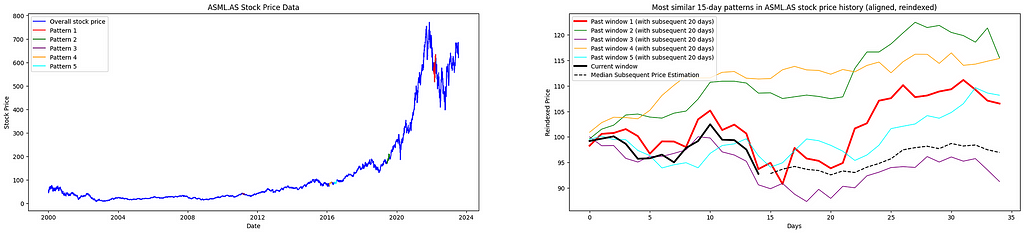
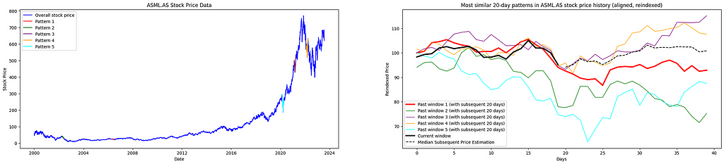
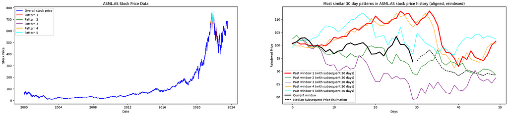
The implemented algorithm identifies and ranks the top five recurring patterns in historical stock price data, arranged from the closest match (Pattern 1) to the least similar among the top five (Pattern 5) in chronological order. By leveraging DTW, the code measures the similarity between time-series sequences, enabling a detailed visual analysis of historical patterns and offering a basis for anticipating potential future price movements.
How Reliable Are These Projections?
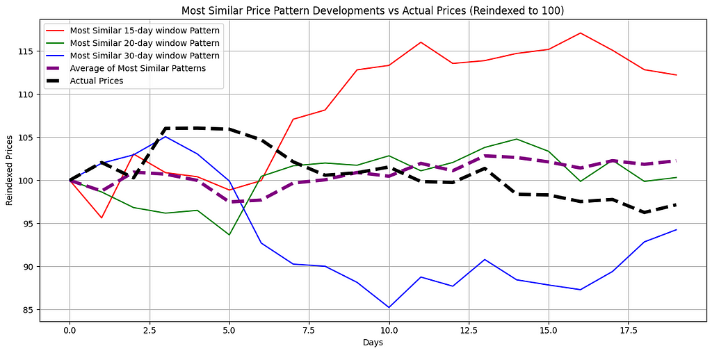
The accompanying graphical analysis delves into the forecasted trajectories derived from the closest-matching historical patterns, as identified through DTW, in comparison to actual price trends. Distinct lines illustrate the average reindexed price developments, based on the most similar historical patterns across varying time window lengths, alongside the actual price trajectory observed for 20 days after the analysis.
A purple dashed line, labeled the “Average of Most Similar Patterns,” represents the mean of various median reindexed price paths. This consolidated metric provides a broader perspective by minimizing anomalies or irregularities in individual patterns, thus yielding a smoother and more cohesive view.
The graphical insights highlight the practical applicability of DTW in uncovering and interpreting patterns within the inherently volatile nature of stock price movements. By comparing projected and actual outcomes, the analysis underlines both the promise and limitations of this method in forecasting price trajectories with historical pattern recognition.
4. Constraints and Potential Enhancements
The capacity to identify recurrent trends in stock price trajectories is crucial for conducting thorough analysis and making well-informed investment decisions. While applying Dynamic Time Warping (DTW) to detect patterns in stock price data, as detailed in this article, demonstrates its utility, it also exposes certain challenges and highlights opportunities for refinement and enhancement.
4.1 Constraints
- Single-Variable Focus: The current DTW implementation emphasizes stock prices as the sole input, neglecting critical factors like trading volume and market volatility. Incorporating these variables could enhance the comprehensiveness of the analysis by providing a broader perspective on market dynamics.
- High Computational Demand: DTW’s quadratic time complexity makes it computationally demanding, especially when applied to large datasets. Analyzing extensive historical stock price data may result in lengthy processing times and substantial resource consumption.
- Reliance on Historical Patterns: The method assumes that historical stock price patterns will reoccur in the future. However, this premise can falter in the highly dynamic and unpredictable nature of financial markets, which are frequently shaped by new, unanticipated factors.
- Susceptibility to Noise: DTW’s vulnerability to noise in the dataset may undermine the accuracy of pattern recognition. Temporary anomalies or price fluctuations can disproportionately influence DTW distance calculations. Implementing smoothing techniques, such as moving averages, can help mitigate these effects and improve accuracy.
4.2 Opportunities for Enhancements
- Optimizing Performance: Techniques like FastDTW, which approximate DTW distances and reduce computational complexity, can be invaluable for handling larger datasets efficiently.
- Minimizing Noise: Employing noise-filtering techniques can help isolate meaningful trends while reducing the effect of transient fluctuations in the data.
- Expanding Features: Integrating additional features, such as volume, volatility, or technical indicators, can significantly enrich the analytical framework and improve the robustness of the results.
- Integrating Machine Learning: Combining DTW with machine learning models could advance its capabilities by merging detailed time-series pattern detection with predictive analytics and validation.
- Multivariable Analysis with DTW: Employing multivariate DTW could enhance the methodology’s scope by analyzing multiple influencing factors concurrently, thereby offering a more holistic analytical perspective.
5. Closing Thoughts
The use of Dynamic Time Warping presents an innovative approach for recognizing and analyzing patterns in historical stock price data. While robust and powerful in many aspects, this methodology also underscores the inherent complexities and multidimensional nature of financial markets.
In an upcoming article, the exploration of pattern recognition methodologies will delve further into the use of Principal Component Analysis (PCA). This expansion will transcend simple price analysis by integrating multiple variables such as trading volumes, market volatility, and a variety of technical indicators. By broadening the analytical focus, the aim is to extract insights that align more closely with the intricacies of market behaviors. Be sure to follow along for future articles!
Automated Grid Trading in Python: A Beginner’s Guide to Algorithmic Profitability
You can save up to 100% on a Tradingview subscription with my refer-a-friend link. When you get there, click on the Tradingview icon on the top-left of the page to get to the free plan if that’s what you want.
➡️Subscribe Me here ➡️ https://medium.com/@ayyratmurtazin/subscribe
I’ve got a lot to share in my upcoming blogs.
Want to get into DeFi yield and airdrop farming? Don’t have time? Don’t know where to start?
Join our newsletter and private group of 300+ DeFi farmers for simple, top 5-minute yield opportunities — plus get our 400+ airdrop database as a bonus!
Unlocking Hidden Trading Opportunities with Python was originally published in The Capital on Medium, where people are continuing the conversation by highlighting and responding to this story.
from The Capital - Medium https://ift.tt/GxfWC1k


0 Comments